Use the free three-observation case when you need to understand what a fill operation changes. Use official documentation when you need to implement a specific operation. Consider the existing Quant Research Project Lab when your gap is organizing a connected investigation rather than choosing a single function.
These resources solve different problems. Buying a project book does not establish the missingness mechanism in your own dataset or make its backtest investable.
Diagnose your gap with a small calculation
Try the missing-price return example before opening the worked answer. Given 100, missing and 110 at three scheduled observations, write what you can infer and what remains unknown. Compare the filled path with a later revealed middle value of 105.
Your deliverable is a one-page note containing the raw observations, endpoint calculation, two competing paths and a treatment decision. If you can explain why equal endpoint returns do not imply equal daily observations, the free case has already achieved its narrow purpose.
Match the resource to the task
| Your task | Start here | What it cannot supply |
|---|---|---|
| Understand zero versus missing | Free worked example | Real vendor field definitions |
| Implement dropping or filling | Official pandas documentation | A justified research policy |
| Explain an actual data gap | Source documentation and authorized clarification | A guaranteed complete history |
| Connect assumptions, evaluation and conclusions | Inspect the existing Research Project Lab | Validated investment performance |
The pandas missing-data guide is freely available. If the unresolved problem is an API parameter, consult the documentation for your installed version before purchasing broader preparation.
Evaluate the actual Lab
Read the public Research Project Lab preview and current product contents. The Lab offers connected synthetic research practice. Inspect whether its workflow helps you make assumptions traceable through the project, rather than assuming it is a market-data cleaning library.
Use the sample to ask three questions: can you identify the input assumptions, can you distinguish a baseline from a changed analysis, and can you explain the limits of a result? If those are your recurring difficulties, a connected project may be more useful than another isolated function example.
The missing-price exercise is separate free material. Do not assume a dedicated imputation module, live market data, vendor support, personal code review or trading recommendations are included. Actual edition contents and availability remain on the product page.
Keep the scope honest
Label synthetic observations and imputed values in any practice artifact. A successful calculation on three invented prices is evidence of that calculation, not evidence of profitable research. When the gap is resolved, continue with a broader project only if it serves your learning task. You can retain the free note and return to research project preparation when you are ready to compare the larger workflow.
Read before choosing
Open the actual pages.
7 sample pages, including complete explanations. No email address or account required.
Open the PDF previewPreview page 4 of 7. Use Enlarge page for a closer view. When the page is focused, use left and right arrows to change pages.
Read the complete free sample as text (7 pages)
Text from the same public sample shown above. Use the page images or PDF for diagrams, equations and original layout.
Sample page 1
QUANT FINANCE PLAYBOOK PYTHON / VALIDATION / RESEARCH Quant Research Project Lab A reproducible synthetic study, three investigations, and a research memo you can defend. QUESTION -> PROTOCOL -> EVIDENCE Keep the failed experiment. EDITION 01 / ORIGINAL PRACTICE & WORKED EXAMPLES
Sample page 2
QUANT FINANCE PLAYBOOK RESEARCH PROJECT LAB Edition 01 / September 2026 02 HOW TO USE THIS BOOK Quant Research Project Lab Ten chapters, three worked capstone investigations, two executable Python scripts, recorded base and extension results, editable worksheets and an annotated research memo. Assumes basic Python and introductory statistics. Read the model before reading the answer. Try each exercise on paper, keep your first attempt, and use the explanation to diagnose the first step that needs repair. Original educational examples The exercises and candidate scenarios are original teaching material. They are not leaked employer questions, employment outcomes, or descriptions of actual trading performance. Sources identify public guidance and further reading; cited organizations do not endorse this publication. Edition 01 September 2026. Independent educational material. This edition has not been reviewed by an identified industry practitioner. Use the supplied companion files alongside the chapters, and distinguish fictional examples and synthetic results from your own evidence. FINAL-SEGMENT MSE / SEED 20260923 Stable 1.161 0.903 Reversed 1.342 2.501 Gray: training-mean baseline. Blue: frozen linear fit. Lower error is better.
Sample page 3
QUANT FINANCE PLAYBOOK RESEARCH PROJECT LAB Edition 01 / September 2026 03 CONTENTS Your route through the work 4 01 / The question before the model 6 02 / Build a world you can inspect 8 03 / Put every value on a time axis 10 04 / Make the simple alternative hard to ignore 12 05 / Freeze a procedure, not just a file 14 06 / Keep the result that did not work 16 07 / Give the decision an accounting rule 18 08 / Three investigations to complete 24 09 / Write a memo that survives a skeptical reader 26 10 / Defend the work and release it cleanly
Sample page 4
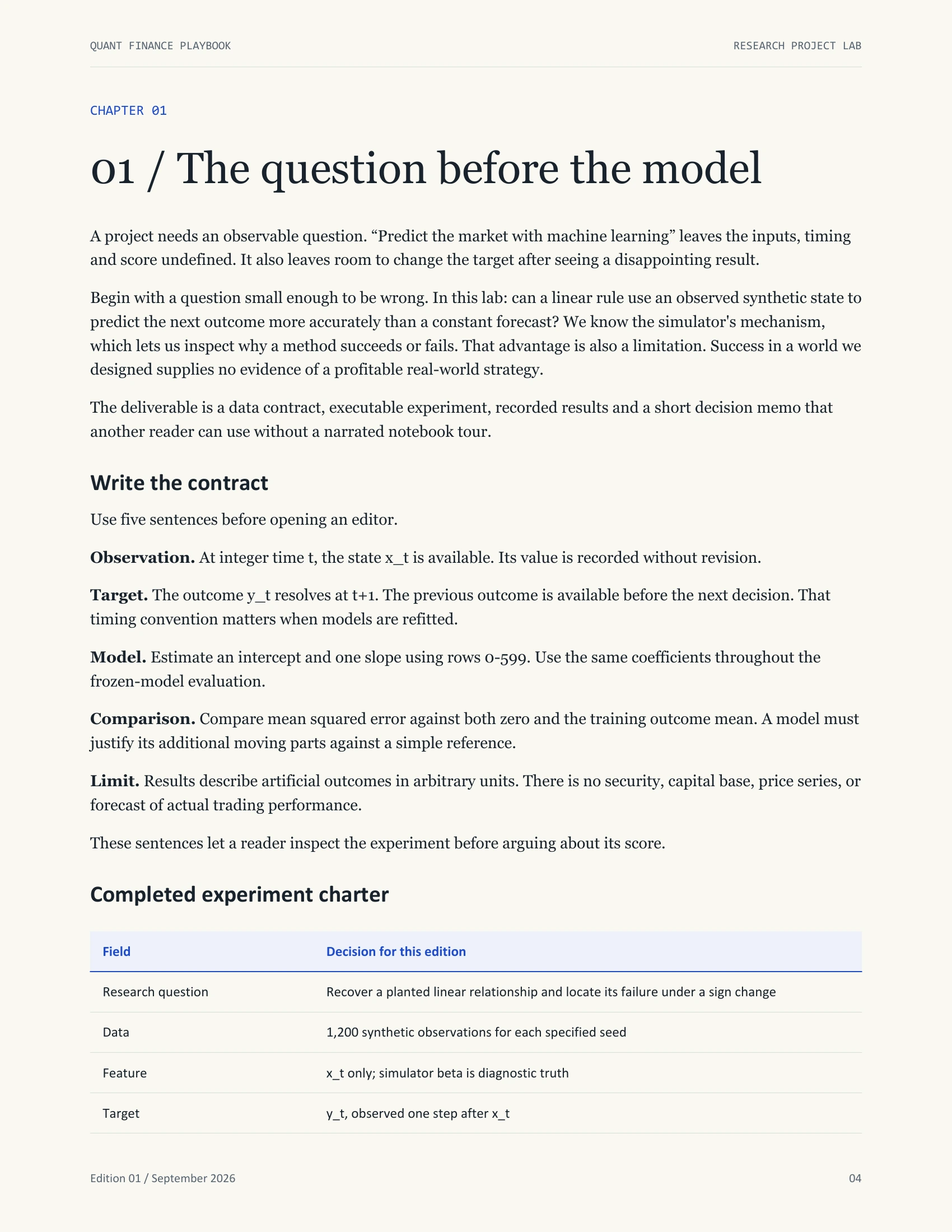
QUANT FINANCE PLAYBOOK RESEARCH PROJECT LAB Edition 01 / September 2026 04 CHAPTER 01 01 / The question before the model A project needs an observable question. “Predict the market with machine learning” leaves the inputs, timing and score undefined. It also leaves room to change the target after seeing a disappointing result. Begin with a question small enough to be wrong. In this lab: can a linear rule use an observed synthetic state to predict the next outcome more accurately than a constant forecast? We know the simulator's mechanism, which lets us inspect why a method succeeds or fails. That advantage is also a limitation. Success in a world we designed supplies no evidence of a profitable real-world strategy. The deliverable is a data contract, executable experiment, recorded results and a short decision memo that another reader can use without a narrated notebook tour. Write the contract Use five sentences before opening an editor. Observation. At integer time t, the state x_t is available. Its value is recorded without revision. Target. The outcome y_t resolves at t+1. The previous outcome is available before the next decision. That timing convention matters when models are refitted. Model. Estimate an intercept and one slope using rows 0-599. Use the same coefficients throughout the frozen-model evaluation. Comparison. Compare mean squared error against both zero and the training outcome mean. A model must justify its additional moving parts against a simple reference. Limit. Results describe artificial outcomes in arbitrary units. There is no security, capital base, price series, or forecast of actual trading performance. These sentences let a reader inspect the experiment before arguing about its score. Completed experiment charter Field Decision for this edition Research question Recover a planted linear relationship and locate its failure under a sign change Data 1,200 synthetic observations for each specified seed Feature x_t only; simulator beta is diagnostic truth Target y_t, observed one step after x_t
Sample page 5
QUANT FINANCE PLAYBOOK RESEARCH PROJECT LAB Edition 01 / September 2026 05 Field Decision for this edition Training 0-599 inclusive Validation 600-899 inclusive Final illustration 900-1199 inclusive Primary score Mean squared prediction error in squared outcome units Baselines Zero and training mean Secondary investigation Bounded positions, turnover costs, one-step delay Failure evidence Worse error than a baseline; unavailable inputs; conclusions sensitive to omitted assumptions Reproduction Python script, recorded version, seeds, hashes, CSV and JSON outputs The “final illustration” was a held-out segment for this fixed experiment. Once this book shows its results, it is no longer unseen evidence for a reader who changes the model after reading them. For your own extension, state that you are exploring this dataset or create a genuinely separate evaluation protocol. A useful project boundary For six available evenings, try this allocation: contract and generator; baselines; time ordering; failure cases; memo; reproduction from the release instructions. Adjust it to the work. If the generator takes longer, reduce the model menu and preserve time to explain the result. Before adding a model or cost assumption, finish the sentence: “This comparison could change my conclusion because…” Exercise: repair the brief Original: “Build an accurate model on a large dataset and use the best result on my resume.” Rewrite it with a target, a decision time, a baseline, and a rule for retaining failed experiments. One defensible answer: “Predict next-step synthetic outcomes from currently observed states; compare a training-only linear fit with the training mean on later rows; preserve all attempted specifications and report the chosen rule's failure under a changed generator.” This does not promise that a model will win. It promises an inspectable investigation. Your first artifact: a one-page charter naming what you observe, when it is available, what becomes known later, your comparator and the result that would change your conclusion. Mark unresolved assumptions explicitly.
Sample page 6
QUANT FINANCE PLAYBOOK RESEARCH PROJECT LAB Edition 01 / September 2026 06 CHAPTER 02 02 / Build a world you can inspect The lab has two random innovations per row. One moves an observed state; the other adds unpredictable noise to its outcome. Write the mechanism as: x_t = 0.65 x_(t-1) + u_t y_t = beta_t x_t + e_t Both innovations have mean zero and variance one and are independently generated. The initial state is zero. The stationary scenario keeps beta at 0.4. The changed scenario keeps it at 0.4 through row 799, then sets it to -0.4. The sign change is specified in the generator; it is not discovered from actual market data. The coefficient 0.65 gives the feature persistence. A high state tends to be followed by another relatively high state, although the next innovation may reverse it. Because its absolute value is below one, an old shock's effect shrinks geometrically: after k steps, its contribution is multiplied by 0.65^k. What the correct model should learn Conditioning on x_t in the stable scenario gives expected outcome 0.4x_t. A linear model with enough data should estimate a slope near 0.4 and an intercept near zero. It will not predict the independent e_t. Even the oracle forecast has expected squared error one because that is the noise variance. Do not reject a finite-sample error below one as impossible. One is the expected error across repeated draws, not a floor on every realized average. Likewise, a fitted slope of 0.405 is not proof that the true mechanism changed. Estimation varies with the sample. In the long-run stationary distribution, the state's variance solves v = 0.65²v + 1. Thus v = 1/(1-0.65²), approximately 1.732. The outcome variance is 0.4²v + 1, approximately 1.277. A zero forecast therefore has expected long-run squared error around 1.277; the oracle improves it by approximately 0.277. Early rows start from zero rather than from that stationary distribution, so this is a reference calculation, not an exact expectation for every finite sample average. Read the generator before the output Open lab.py and find the generate function. It constructs x first and y second. The order encodes the information structure. The beta value is stored to explain the experiment later; it must never be provided to the fitted forecasting rule. The code uses a local random.Random(seed) instance. Each experiment therefore starts with its own generator state. It does not depend on random calls made by unrelated notebook cells. Recording a seed is useful only when the algorithm and environment are also known. The output records the Python version and script hash; the release run used Python 3.12.14.
Sample page 7
QUANT FINANCE PLAYBOOK RESEARCH PROJECT LAB Edition 01 / September 2026 07 Changing the regime flag does not change the sequence of random shocks for a given seed. It changes how the same state is mapped into an outcome after row 799. This pairing helps isolate the effect of the sign change. It does not produce two independent datasets, so do not count them as independent evidence when discussing uncertainty. Data dictionary Column Meaning Available to model? t Ordered decision index Yes, as an index; this model does not use it as a predictor x Current observed state Yes y Outcome resolving next step Only as a previously resolved training label beta Generator's current signal coefficient No; diagnostic truth All numeric outcome units are arbitrary. Calling 0.27 a “27% return” would invent a denominator and an economic interpretation. A synthetic decision exercise can teach accounting without masquerading as a backtest of a traded instrument. Exercise: change one assumption Suppose u_t has variance four rather than one. Keep e_t variance one and all coefficients unchanged. What happens to the long-run state variance and the oracle error? Solution. State variance becomes 4/(1-0.65²), approximately 6.926. The oracle still removes the conditional mean and leaves e_t, so its expected error remains one. The zero forecast becomes worse because the predictable component has become more variable. A larger percentage improvement need not mean a more sophisticated model; the data-generating problem became easier relative to its noise. Exercise: explain what is missing Name three reasons success here would fail to establish a live trading opportunity. Discussion. We chose a known, simple signal; there is no market impact or order execution; no data licensing, revisions, selection of securities, capital constraints or competition is modeled. Many other answers are valid. State what each omission changes rather than appending a generic limitations paragraph.